Given that the error correction of quantum systems is a formidable challenge, it would seem a basic question to ask how long is it possible to leave an unknown quantum state for before we can no longer sucessfully error correct it (when it experiences errors from within a given class)? Motivation comes from the classical wqorld where hard drives and USB sticks work great for storing data. They don't need regular error correction, they're not even powered. The data just sits there, stable, for ever (to all intents and purposes). Why not for quantum data?

The first thing that we do is find the best possible physical representation of a qubit, i.e. we find the two level system with the longest possible decoherence time. That's a good start, but what if we want to store the state for longer than that? The only option is to encode your logical qubit across multiple physical spins. If a little bit of encoding gives you a longer survival time, then it's reasonable to expect that more encoding gives you more benefit. So, what we're trying to do is find an encoding that gives a storage time that increases with the number of physical spins used, N. Ideally this time should grow exponentially with N, but we would tolerate a polynomial increase. We consider a logarithmic increase as probably being insufficient because that doesn't even give you long enough to get the state encoded! This distinction already makes thermodynamic considerations insufficient - there are some results that state that the given memory model is stable in the limit of large system size. That could just mean logarithmic.

If we're not allowing any error correction (remember, it's a question of how long can we go between rounds of error correction), what abilities do we have to prevent/remove errors? The only ability that we have is to specify the intrinsic interactions of the physical spins, i.e. their Hamiltonian. Our aim is therefore to specify the encoding and the Hamiltonian in such a way that, for a given class of errors, the Hamiltonian prevents the errors from building up in such a way that there is a false correction of the encoded state at the end.

What sort of errors is it that we're trying to protect the system against? Ultimately, there are a number of issues that we have to take care of:

1. Imperfect preparation of the initial encoded state.
2. Imperfect implementation of the system Hamiltonian, modelled by an unknown weak perturbation to the intended implementation.
3. External noise during storage, modelled by an external bath which is in a low temperature state of the bath Hamiltonian, and is weakly coupled to the system.
4. Measurement errors when applying the syndrome measurements for error correction.

I'm choosing to concentrate on the second point, because taking it into account automatically leads you to considerations that at least partially tackle the first and last aspects. Also, a proper proof of protection against unknown perturbations will most likely be extensible to a system coupled to a zero temperature environment, and from there, adding temperature is not infeasible. This would ultimately lead to proofs that don't require restrictive assumptions about the environment, such as Markovianity. It is important to emphasise two aspects. Firstly, this is not a solved problem. Many people claim that it is, but they have missed the point. I'll point out that point as we go through. Secondly, an even broader set of physicists are happy with statements such as "encode in the ground state of a gapped Hamiltonian, and the gap protects you". A gap helps, but it's nowhere near enough.

Given that we're talking about a dual process of choosing an encoding and a Hamiltonian, what's the connection? A natural choice is to encode the two logical states of the qubit as eigenstates of the Hamiltonian. So, let's draw some simple conclusions about the nature of the eigenstates and their energies.

• The chosen eigenstates should be degenerate: Consider choosing two eigenstates that are separated by energy E. An initial state $\alpha\ket{0}+\beta\ket{1}$ evolves, after time t to $\alpha\ket{0}+\beta e^{-itE}\ket{1}$. That's no problem because we know the Hamiltonian and the time that it's evolved for, so part of the error correction process can involve removing the phase. However, a perfectly reasonable error in the Hamiltonian is to make everything a bit too strong, so instead of $H$, we make $(1+\delta)H$ for some small value of $\delta$. Now after time t, because we don't know the value of $\delta$, we can't compensate for it and we're left with an extra phase factor $e^{i\delta tE}$. After time $\pi/(\delta E)$, this constitutes a logical phase gate which error correction can't correct for. Hence, the survival time is upper bounded by $\pi/(\delta E)$, so to get a survival time that scales with the system size, E must vanish with the system size and, preferably, E=0. It then makes sense to make the eigenstates the ground states if the system.

• Topology is necessary: So far, we have not mentioned what are a reasonable class of perturbations. In practice, Hamiltonians and their perturbations will consist of a sum of spatially local terms. Now, assume that the two logical states $\ket{0}$ and $\ket{1}$ are distinguishable by some local operator. One can implement this observable in the form of a local perturbation that gives a (small) relative energy shift between the two states. Hence, similarly to the previous argument, after a time $\pi/\delta$, a logical error can be induced. In order to avoid this, the two degenerate eigenstates must be locally indistinguishable. This is the definition of topological order.

A typical example of a system with topological order is the Toric Code in 2D. After briefly introducing this code, we'll illustrate the issues that one has to worry about for a quantum memory using this code.

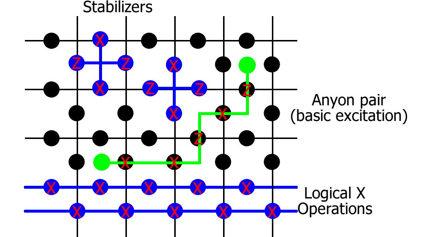
The Toric code is the quintessential example of a planar code; one which can be defined for arbitrarily many qubits with a correspondingly increasing code distance, and which has a finite fault-tolerant threshold without requiring the additional complications of concatenation. I typically consider a version which is rotated relative to the standard description, as this has better symmetry properties. Unless I explicitly make statements about the non-rotated version, results quoted here are for this rotated version. Starting from an $N\times N$ square lattice with periodic boundary conditions, place a qubit in the middle of each edge. For each vertex $v$ and face $f$ of the lattice, there are four neighbouring qubits, two on horizontal edges $E_H$ and two on vertical edges $E_V$. The corresponding stabilizers are defined as $$ K_v=\prod_{e\in E_H}\!\!Z_e\prod_{e\in E_V}\!\!X_e,\; K_f=\prod_{e\in E_H}\!\!X_e\prod_{e\in E_V}\!\!Z_e. $$ (For the non-rotated version, the vertex and face terms are just a tensor product of 4 X or Z rotations respectively.) All terms mutually commute, which is what makes this model relatively simple to manipulate, and each has eigenvalues $\pm1$. The space of Toric code states $\ket{\Psi_{ij}}$ for $i,j\in\{0,1\}$ are defined by the relations $K_v\ket{\Psi_{ij}}=\ket{\Psi_{ij}}$ and $K_f\ket{\Psi_{ij}}=\ket{\Psi_{ij}}$ for all $v,f$. There are $2N^2$ qubits and $2N^2-2$ independent stabilizers, leaving a four-fold degeneracy (the indices $i,j$) that represents two logical qubits, for which the logical Pauli operators correspond to long-range operations along a single row or column, looping around the entire torus. The logical $Z$ operators are two inequivalent loops of Paulis along a row; one made up of $X$ rotations along a set of horizontal edges and the other $Z$ rotations along a set of vertical edges. The logical $X$ operators similarly utilise rotations on two different columns. Starting from a logical state $\ket{\Psi_{ij}}$, and applying continuous segments of $X$ and $Z$ operators, it is possible to form closed loops (meaning that all stabilizers return $+1$ expectation). Provided those loops are topologically trivial (i.e.\ they don't form loops around the torus), the state is the same as the original one while non-trivial loops correspond to logical errors. This degeneracy of the code means that if a large set of errors has arisen, it is not necessary to establish from the locations of the anyons exactly which errors occurred in order to correct for them; one only has to form the closed loops which are most likely to be trivial.

The corresponding toric code Hamiltonian is defined by $$ H=-\sum_n\Delta_nK_n, $$ meaning that the ground states are $\ket{\Psi_{ij}}$, and excited states have an energy gap of at least $2\min_n\Delta_n$, where $\Delta_n>0$.

In order to error correct the Toric code, one first measures the error syndrome by measuring the stabilizer operators $K_n$, getting a value $\pm 1$ for each measurement. There must be an even number of $-1$ values, and each of these is described as a virtual particle called an anyon. Anyons can be moved around the lattice by suitable application of X and Z rotations, and when anyon pairs meet up, they fuse together, removing both anyons from the system (thereby reducing the number of -1 stabilizers, and taking us closer to the ground state space. Error correction proceeds by trying to interpret from the positions of those anyons which error is most likely to have occurred, and then performing that pairing in order to remove the errors. Once all the stabilizers are back to a +1 value, we have paired up all anyons, and they were either paired up by trivial loops that did not extend around the torus, in which case we have sucecssfully corrected the system, or non-trivial loops have been implemented and the error correction fails because the data can no longer be trusted.

It turns out that the topological phase, i.e. the ground state space, is remarkably stable to perturbations. The precursor of the argument is very clear, stemming from perturbation theory. Imagine you introduce a small perturbation $$ V=\delta \sum_nX_n, $$ and you ask how the ground state energies change under the perturbative expansion. Since one must implement a loop of at least N X operators around the lattice in order to take one ground state to an orthogonal one, the leading order splitting in ground state energy is only $O((|V|/\Delta)^N)$, i.e. as the lattice increases in size, we get an exponentially good stability. Moreover, if a quantum state is encoded in the degenerate ground state space, it must surivie a time $O((\Delta/|V|)^N)$. Perfect!

However, I called this a precursor argument because one has to be very careful about the range of applicability of the result - it requires $|V|\ll\Delta$, but $|V|=2N^2\delta$, and we really want to be working in the regime $\delta\ll\Delta$, not $N^2\delta\ll\Delta$. Nevertheless, these results have recently been extended to work in this more desirable regime.

Initial mis-readings of the original argument (which was never explicit enough about what constituted a sufficiently weak perturbation), and subsequent derivation of this new result has lead people to believe that the issue of stability of codes such as the toric code under the influence of perturbations is a resolved question. It is not. When I made the argument about the stability of the memory, I was very careful to specify that the memory had to be encoded in the ground state space. Why is this important? Well, while the ground state energy might not change very much, such as in high order perturbation theory, the ground state space itself changes even at first order. If we don't know what the perturbation is, we don't know how the ground state space has changed, and we don't know how to encode it. So, there could still be issues to answer with regards to the stability of topological encodings.

Given that we don't know the perturbation, there seem to be a couple of different ways that one could proceed. Ideally, we want to encode in the perturbed ground state space, and one can do that by using an adiabatic path to perform the encoding. However, we still don't know how to perform error correction in the perturbed space in order to ensure that the state we've produced is correct, or to output it after the storage. Adiabatic paths tend to introduce errors determined by the speed at which the preparation is performed (and in the presence of perturbations, one has to go slower than expected!), and those errors can be problematic (and need a similar treatment to what I will consider in the following). Moreover, that's only suitable for the initial preparation of the state. Realistically, we're still looking at preparing the state once, and then performing many rounds of error correction, and we're just wanting to know how much we can space out those rounds. So, really, we're more interested in the second method, which is providing an intial state in a space with a known error correction protocol, i.e. one drawn from the original, unperturbed ground state space. This is the assumption that I consider the most relevant.

Now, since our encoding is probably not an eigenstate of the perturbed Hamiltonian, it evolves in time, potentially doing bad things, but how long have we got until something irreparable happens? There are two natural instances to ask this question in. For both, we limit the set of possible perturbations to being a set of weak, local operations (each local term of norm no more than $\delta$). Firstly, one can ask "What is the worst perturbation that I can construct?" This gives you some idea of how stable or not the memory is, but you might level the criticism at it that it's a really bizarre perturbation that's extremely rare in practice, so you ask the second question of "What is the behaviour under typical perturbations, such as a uniform magnetic field". It turns out that the answer to both questions is that the survival time is no more than logarithmic in N when one assumes that all the $\Delta_n$ are equal (the most obvious choice). Armed with suitable understanding, one can then proceed to assess how things have to be changed in order to get a more stable memory.

As a first step to creating an evil perturbation that destroys the stored information as quickly as possible, let's start with a simple proof of principle that bad things can indeed happen. We'll do this by composing two different perturbations, one which creates an anyon pair locally, and one which propagates one of the anyons around a non-trivial loop.

The first of these perturbations invokes a really neat trick. Consider an initial Hamiltonian $H$, and define a perturbation $$ V_1=UHU^\dagger -H $$ where $U$ is a tensor product of single-qubit rotations on any subset of qubits, where the rotation is only about some small angle $\epsilon$. These restrictions ensure that $V_1$ does indeed have the required properties of a local perturbation. Moreover, the changes are really easy to analyse because $H+V=UHU^\dagger$, so the new eigenstates are just the rotation $U$ applied to the original eigenstates. Each local rotation introduces a local anyon pir with probability amplitude $\sin^2\epsilon$. Of course, such a probability is small, but repeated $O(N)$ times down one dimension of a lattice, for example, means that we can have approaching 50% probability of having an odd number of anyon pairs, which, after evolution under our second perturbation, will each have been converted into a logical error.

I'm not going to detail how to make the second perturbation, $V_2$. Suffice it to say that one can design local Hamiltonian terms of the form $$ X_n(\identity-K_nK_{n+1}) $$ that propagate an anyon from one site to the next (the site $n$ if the site where the two stabilizers $K_n$ and $K_{n+1}$ meet), and the effective Hamiltonian in the single anyon subspace maps exactly into a tridiagonal matrix. This means that we can borrow results from perfect state transfer to learn how to perfectly propagate an anyon as quickly as possible around the loop. It takes time $O(N/\delta)$ when each term has bounded norm $\delta$.

If $H$ is our original toric code Hamiltonian, these two techniques can be combined into a single perturbation $$ V=U(H+V_2)U^\dagger-H $$ such that after time $O(N/\delta)$ there is a prbability of 50% of the code being subject to a logical error.

A linear time does not seem so bad, but this is just for a configuration where we create a single column of anyon pairs and propagate them around rows. Different configurations can shorten this time. For example, numerics suggest that by spacing columns of anyon pairs by a constant amount (and hence only propagating each anyon by a constant amount), error correction can fail after a constant time. However, this has never been rigorously proven, and the strongest result that we managed to realise was that a designer perturbation can destroy the stored information in a time $O(\frac{1}{\delta}\log N)$.

Let's now consider what happens when we put a magnetic field $\sum_n\delta_n X_n$ on the (rotated) toric code, and evolve the unperturbed ground state (incidentally, this is what is referred to in condensed matter as an instantaneous quench). Perhaps a more typical case is less destructive. I won't go through the full derivation, that's what the paper's for, but what one can do is analyse the system and bound the survival time for any possible set of field strengths $\delta_n$. This is done by mapping to many parallel copies of a model called the transverse Ising model in 1D with periodic boundary conditions. $$ H_I=\sum_{n=1}^N\Delta Z_nZ_{n+1}+\sum\delta_nX_n $$ We start this system in the all zero state, and demand the time at which there is a finite probability that more than half the spins have flipped to the 1 state. It turns out that we can relate this to the magnetisation $$ M(t)=\bra{\Psi(t)}\frac{1}{N}\sum_{n=1}^NZ_n\ket{\Psi(t)}, $$ so that $M(0)=1$. If $M(t)$ drops within $O(1/\sqrt{N})$ of 0, we can no longer guarantee that the memory is stable (assuming we know that the errors are all X-type. If not, the threshold is some positive value roughly 0.56, see next section.) We can analytically prove bounds on the generic behaviour of this magnetisation. Starting from value 1, it drops exponentially for a time $O(N/\delta)$. For sufficiently small N, this appears like a linear drop with gradient $\max_n\delta_n^2/\Delta^2$, and the magnetisation never drops to a critical level, and the memory remains stable. As the system size gets bigger, the exponential tending towards 0 takes over, and the memory is only stable for a time $O(\frac{\Delta^2}{\delta^3}\log N)$.

The figure below illustrates the behaviour of the magnetisation for a unform magnetic field, $\delta_n=\delta$ which, up to numerical constants, saturates the bound. 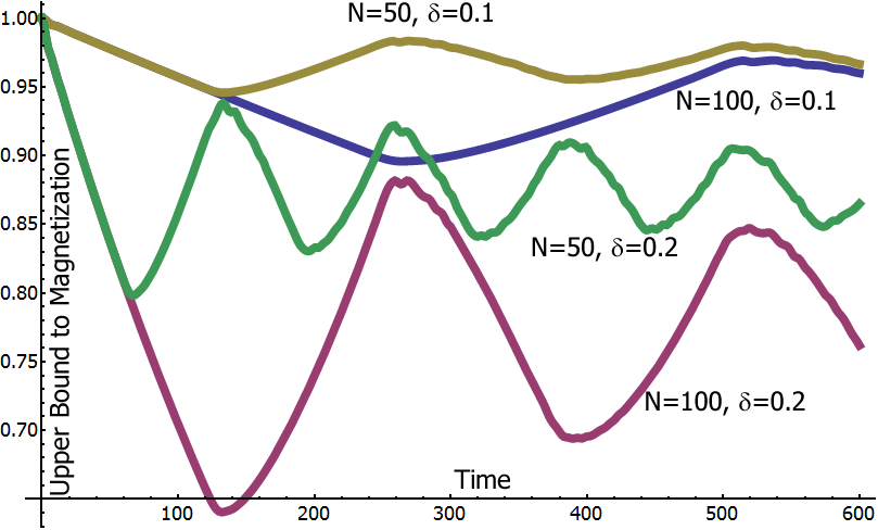This is clearly bad news - the toric code Hamiltonian is not sufficiently stable against unknown uniform magnetic fields. What went wrong? The problem is that once a single error has been created (which requires some energy, and therefore only occurs with small probability on a given site), it doesn't cost any more energy to create a second error on a neighbouring site, and hence to propagate these errors around a loop. Of course, this is exactly what happened in the designer example above.

A way to avoid this is to change the constants $\Delta_n$ at each site, or change the structure of the code such that anyons have to take a path of increasing energy before they can perform a non-trivial loop. It seems unlikely that this second option can be achieved in two spatial dimensions (although three dimensions look promising), but we can change the $\Delta_n$. One good idea is to learn from condensed matter physics. There, they're plagued by a problem known as Anderson localisation wherein random impurities prevent conduction in a metal. This prevention of transport is exactly what we need - if we randomise the $\Delta_n$, one can deliberately induce Anderson localisation, and prevent the anyons from propagating around the lattice in almost all instances. A numerical example is shown below, leaving in the original case of no randomness for comparison. One can analytically prove that in almost all cases, the survival time of the memory improves exponentially, giving a polynomial in N.

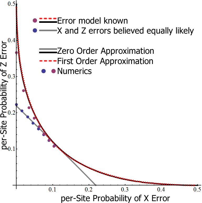
If we are to ascertain how long a memory can last between rounds of error correction, it is important to understand how that error correction performs, and what levels of noise it can tolerate. There is an elegant construction that maps the threshold for error correction of local noise in the toric code into the temperature of the phase transition of the random bond Ising model (RBIM). If syndrome measurements are perfect, it maps to a pair of 2D RBIM systems. In the case of the non-rotated Toric code, X errors map to one system and Z errors to the other. This means that the threshold is given in terms of $\max(p_X,p_Z)$. However, the rotated version has the two systems identical with vertical bonds corresponding to Z errors and horizontal bonds corresponding to X errors. This is much more tolerant of asymmetries in the error rates. Imperfect measurements introduce a third dimension to the model (with probabilities of the signs of the couplings in the third dimension corresponding to probabilities of a measurement error). While the error thresholds are severely reduced, they remain finite nonetheless.

An important feature of the mapping is that in order for the code to perform at its optimum, it needs to know precisely what the error model is. In our present scenario, where we don't know the perturbation, we obviously don't know the error model, and just have to guess based on some basic properties that we can extract such as the probability that measurement of a stabilizer gives a value $-1$. This implies an error rate, and, without further information, we assume the $p_X=p_Z$. How badly does this mess up the error correction threshold? Even for local noise models, it can significantly skew things (see below), but it could be even worse in a perturbed system in which errors can also be spatially correlated.

We understand quite a lot about the performance of the toric code as a memory under the influence of unknown perturbations. I believe there are still gains to be made by studying the Anderson Localisation problem further. A more careful derivation should be able to prove longer storage times. However, the more interesting direction is to prove necessary and sufficient conditions for a memory to be protected against unknown perturbations. We can then examine whether any known models satisfy these constraints, and start to expand the proofs in the direction of weakly coupled environments.

1. A. Kitaev, Annals Phys. 303, 2 (2003).
2. F. Pastawski, A. Kay, N. Schuch and I. Cirac., Quant. Inf. Comput. 10, 580 (2010).
3. A. Kay, Phys. Rev. Lett. 102, 070503 (2009).
4. A. Kay, Phys. Rev. Lett. 107, 270502 (2011).
5. A. Kay, arXiv: 1208.4924